What is TensorFlow?
TensorFlow is an open-source machine learning framework developed by Google. It was released in 2015 and has since become one of the most popular frameworks for building and training machine learning models.
TensorFlow is used in a wide range of applications, including image recognition, natural language processing, and speech recognition. It is also used by companies like Google, Uber, and Airbnb to power their machine learning systems.
How to get started with TensorFlow?
First of all we need to install TensorFlow. There are two ways to do this: using pip or using Docker.
Installing TensorFlow using pip
To install TensorFlow using pip, run the following command in your terminal:
pip install tensorflow
To check if TensorFlow is installed correctly, run the following command in your terminal:
python -c "import tensorflow as tf; print(tf.__version__)"
Installing TensorFlow using Docker
To install TensorFlow using Docker, run the following command in your terminal:
docker pull tensorflow/tensorflow
To check if TensorFlow is installed correctly, run the following command in your terminal:
docker run -it --rm tensorflow/tensorflow python -c "import tensorflow as tf; print(tf.__version__)"
Loading the MNIST dataset
Once TensorFlow is installed, you can start using it to build and train machine learning models. For this tutorial we are going to use the MNIST dataset, which contains images of handwritten digits. The goal is to build a model that can recognize these digits.
First, you need to import TensorFlow and load the MNIST dataset:
import numpy as np
import pandas as pd
import matplotlib.pyplot as plt
from tensorflow import keras
import tensorflow as tf

(x_train, y_train), (x_test, y_test) = keras.datasets.mnist.load_data()
Notice that we are using the Keras API to load the dataset. This is because Keras, which was a separate project, is now part of TensorFlow and provides a more user-friendly interface for building and training machine learning models.
Let’s take a look at the shape of the dataset:
print("x_train shape:", x_train.shape, "y_train shape:", y_train.shape)
print("x_test shape:", x_test.shape, "y_test shape:", y_test.shape)
# x_train shape: (60000, 28, 28) y_train shape: (60000,)
# x_test shape: (10000, 28, 28) y_test shape: (10000,)
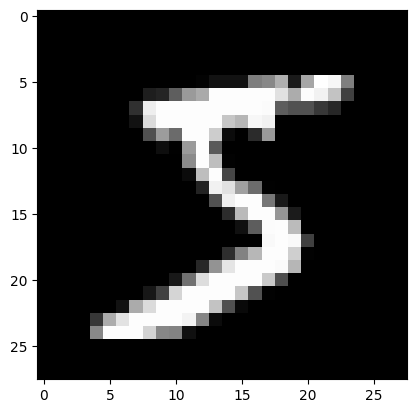
As you can see, the dataset contains 60,000 training images and 10,000 test images. Each image is a 28x28 pixel grayscale image. The labels are integers between 0 and 9, which correspond to the digits 0 to 9. Let’s take a look at some of the images:
img_index = 0 #change the number to display other examples

first_number = x_train[img_index]
plt.imshow(first_number, cmap='gray') # visualize the numbers in gray mode
plt.show()
print(f"Correct number: {y_train[img_index]}")
# Correct number: 5
Preparing the data
Before we can train our model, we need to prepare the data. This involves converting the images into a format that can be used by the model. We also need to normalize the data so that the values are between 0 and 1.
x_train = x_train.reshape(-1, 28, 28, 1)
x_test = x_test.reshape(-1, 28, 28, 1)

x_train = x_train.astype('float32') / 255
x_test = x_test.astype('float32') / 255
Building the model
Now that the data is ready, we can start building our model. We will use a convolutional neural network (CNN) for this task. CNNs are a type of neural network that are commonly used for image recognition tasks.
model = keras.models.Sequential()
model.add(keras.layers.Conv2D(64, (3, 3), activation='relu', input_shape=(28,28,1)))
model.add(keras.layers.MaxPool2D(2, 2))

model.add(keras.layers.Conv2D(64, (3, 3), activation='relu'))
model.add(keras.layers.MaxPool2D(2, 2))

model.add(keras.layers.Conv2D(64, (3, 3), activation='relu'))
model.add(keras.layers.MaxPool2D(2, 2))

model.add(keras.layers.Flatten())
model.add(keras.layers.Dense(64, activation='relu'))

model.add(keras.layers.Dense(32, activation='relu'))

model.add(keras.layers.Dense(10, activation='softmax')) #output are 10 classes, numbers from 0-9

# Print model summary
print(model.summary())
Ouput:
Model: "sequential"
_________________________________________________________________
 Layer (type)                Output Shape              Param #
=================================================================
 conv2d (Conv2D)             (None, 26, 26, 64)        640

 max_pooling2d (MaxPooling2D  (None, 13, 13, 64)       0
 )

 conv2d_1 (Conv2D)           (None, 11, 11, 64)        36928

 max_pooling2d_1 (MaxPooling  (None, 5, 5, 64)         0
 2D)

 conv2d_2 (Conv2D)           (None, 3, 3, 64)          36928

 max_pooling2d_2 (MaxPooling  (None, 1, 1, 64)         0
 2D)

 flatten (Flatten)           (None, 64)                0

 dense (Dense)               (None, 64)                4160

 dense_1 (Dense)             (None, 32)                2080

 dense_2 (Dense)             (None, 10)                330

=================================================================
Total params: 81,066
Trainable params: 81,066
Non-trainable params: 0
In the above code, we have defined a CNN with three convolutional layers and two fully connected layers. The first, second and third convolutional layer has 64 filters with a size of 3x3. The first fully connected layer has 64 neurons, the second fully connected layer has 32 neurons, and the output layer has 10 neurons, one for each digit.
Training the model
Now that the model is built, we can train it using the MNIST dataset. We will use the Adam optimizer and the categorical cross-entropy loss function.
model.compile(optimizer='adam',
    loss='sparse_categorical_crossentropy',
    metrics=['accuracy'])

history = model.fit(x_train, y_train, epochs=5)
Ouput:
Epoch 1/5
1875/1875 [==============================] - 46s 18ms/step - loss: 0.2180 - accuracy: 0.9318
Epoch 2/5
1875/1875 [==============================] - 29s 16ms/step - loss: 0.0718 - accuracy: 0.9784
Epoch 3/5
1875/1875 [==============================] - 28s 15ms/step - loss: 0.0549 - accuracy: 0.9836
Epoch 4/5
1875/1875 [==============================] - 27s 15ms/step - loss: 0.0416 - accuracy: 0.9869
Epoch 5/5
1875/1875 [==============================] - 29s 15ms/step - loss: 0.0354 - accuracy: 0.9894
Evaluating the model
Now that the model is trained, we can evaluate it on the test set.
model_loss, model_accuracy = model1.evaluate(x=x_test,y=y_test)
print(f"Loss: {model_loss}, Accuracy: {model_accuracy}")
Output:
313/313 [==============================] - 3s 9ms/step - loss: 0.0553 - accuracy: 0.9851
Loss: 0.055307190865278244, Accuracy: 0.9850999712944031
Making predictions
Now that the model is trained, we can use it to make predictions on new images. Let’s take a look at some examples:
predictions = model1.predict(x_test)

print(f"Predicted value: {np.argmax(predictions[img_no])}")
Output:
313/313 [==============================] - 3s 9ms/step
Predicted value: 7
Conclusion
In this tutorial, we have learned how to build a convolutional neural network (CNN) using Keras and TensorFlow. We have also learned how to train the model and evaluate it on the test set. Finally, we have learned how to make predictions on new images.